The Data
import numpy as np
import pandas as pd
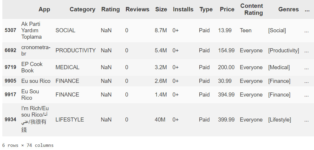
df_raw = pd.read_csv('googleplaystore.csv')
df_raw.head()
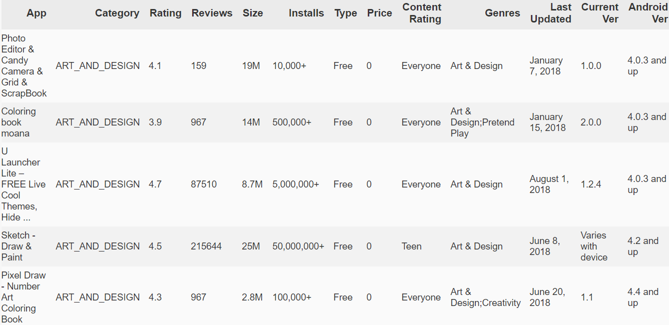
To sum it up, this is App data scraped from GooglePlay store including Price, Content Genre, Size, number of installations, etc. One thing you could do with this dataset is develop a model to predict installs or app rating based on this data, which we'll do later on, but first I want to just take a minute here to assess the power of pure intuition and what can be done with just a tiny bit of EDA.
EDA Step 1 - Intuition
First of all, just by looking at column headers we can make a few guesses as to where we might start looking for intervariate relationships, correlations to any variables we might want to predict for, potential confounding factors, etc.
For example, we know from experience that we, and users in general, are more likely to try installing a free app - ceteris paribus - over a paid app. However at the same time we understand that while not always the case, there is often an increase in quality (or content quantity, e.g. lite vs. full versions) when we go from free to paid apps.
These may seem like obvious statements, but if you think about it for a moment our intuition as human beings with a lifetime of experiences is really quite powerful. Without employing any software or code we have at least one clear starting point from which to begin our data exploration and analysis. In this and other projects I'll surely come back to this simple point, but we immediately see the difference between a human analyst with intuition and a hypothetical analyst who only knows how to run code and build models. Things like common sense, past experience, and intuition will give us a huge jump on any analytical task if we take some time to think rather than jumping immediately into the code.
df_raw.info()
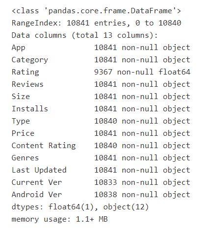
Getting back to this particular dataset, here are a few examples of observations we can make before needing to dig any deeper:
- Category, Type, Content Rating will definitely be our categorical variables. Genres we'll eventually need to look at one-hotting everything as well. It's basically a bunch of T/Fs where each app can have one or more genres
- Last Updted we'll change to a Date type. may or may not be useful. Probably apps that have NOT been update in a long time won't be a popular, whereas apps that have been updated any time in the fairly recent past will probably not vary too much based purely on the difference in date (i.e. 1 week ago and 2 weeks ago may not prove to be all that different on average, whereas over a year ago would be a red flag). don't know if it'll be necessary but it might be an option to group these last updateed dates into categories representing how (in)active the devs are.
- Reviews: more reviews tends to mean more popular, widely used apps. Also let's be honest you're more likely to download an app with 12000 testimonials than a similar looking one with 12 (or none).
- Size: I think this might be mixed. Smaller generally would be better all else equal but larger apps can potentially do more and have higher quality. Plus larger sizes just might be necessarry for certain categories. I think we'll see sizes grouped by app category in the data, so size alone might not be all that telling and may end up being a proxy for things like category and price
Again, for my full annotations please check out the original notebook on github.
EDA Step 2 - Univariate Inspections
# Useful Python3:

DATAFRAME.head(), .tail()
DATAFRAME.info()
DATAFRAME.dtypes(), numpy.dtype()
DATAFRAME.describe()
DATAFRAME.isnull().sum()
DATAFRAME.loc[], .iloc[]

pd.unique(SERIES)
SERIES.value_counts(), SERIES.value_counts().plot('bar')
np.mean(SERIES), np.stdDev(SERIES), np.median(SERIES)
SERIES.quantile()

SERIES.plot.density()
plt.hist()
plt.boxplot()
sns.catplot()
sns.countplot()
Once we've spent some time imagining where we might be headed and jot down any preliminary notes, we can start looking at a few things for each variable we have, namely:
- Data types; what they are, whether they make sense, maybe they've just been coerced in data preparation, for instance
- Categorical vs. Numeric variables
- Unique values & value counts (for categoricals)
- Numeric variable distributions
You could jump right into something like a correlation matrix, but so long as the data isn't superbly sparse or anonymized I like to get a feel for each variable individually and assess any oddities that may have been introduced in data collection and preparation (taken as exogenous processes for this project).
For example,
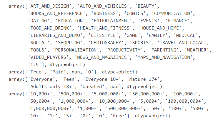
categoricals = ['Category', 'Type', 'Content Rating', 'Installs']
for c in categoricals:
	print(pd.unique(df_raw[c]))
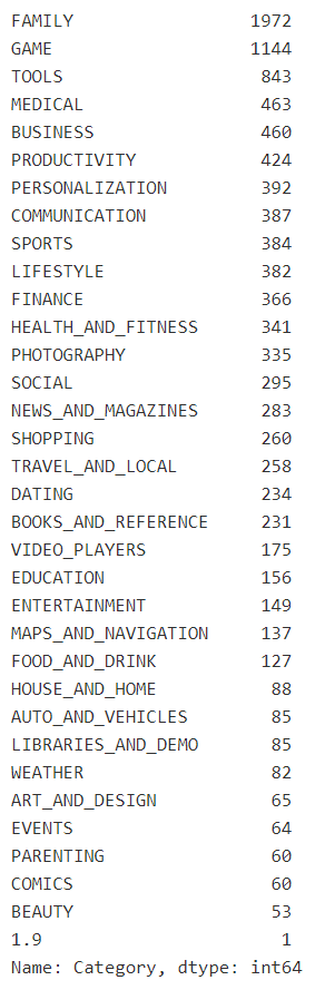
df_raw.Category.value_counts()
So as long as we have visible data (as opposed to hashed data, for instance), one approach is to separate variables into numeric and categorical, and then review/clean them up one by one, though obviously checking back in on the data as a whole when investigating discrepencies or mistakes in the data.
Univariate Inspection Example - App Category
For instance in the GooglePlay data when checking out App "Category', we come across one row where category is suddenly just '1.9'. In this case we need to take a step back and look at the surrounding data in order to understand why we have this value.
df.loc[df['Category'] == '1.9']
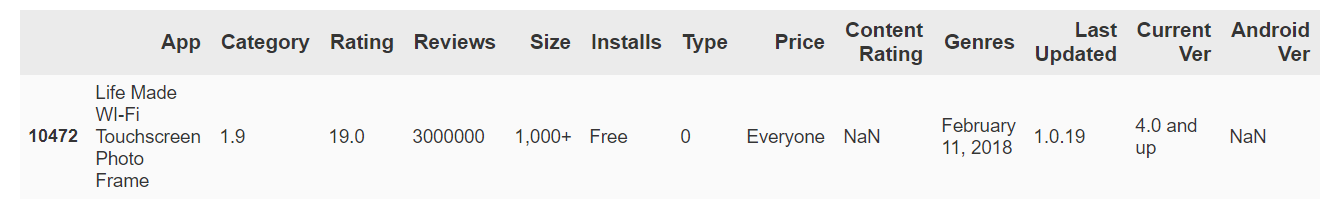
Looking this app up on the Google Play Store, the category is in fact 'LIFESTYLE'. And then we can see that every other value after Category is shifted one to the left for some reason, probably just a mistake coming from the original data.
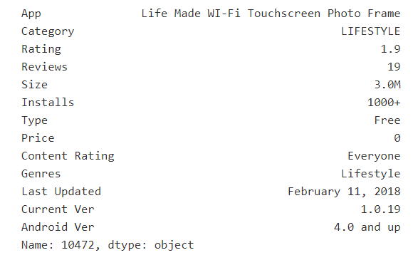
But regardless, this is another situation where being a logical human analyst (and being thorough) comes in handy, seeing as we can just look at the other values in the same row and shift it all, rather than throwing up our hands and dropping instances of Category=='1.9' without digging deeper. Not so significant when it's just one row, but taking a step back and making small, common sense decisions proves to be important in the long run when you have messier data than this.
df.iloc[10472] = ['Life Made WI-Fi Touchscreen Photo Frame', 'LIFESTYLE', 1.9, 19, '3.0M', '1000+', 'Free', 0,  'Everyone', 'NA', 'February 11, 2018', '1.0.19', '4.0 and up']
df.iloc[10472]
In addition to general data cleaning and weeding out inconsistencies, EDA step 2 is where I like to do my first visualizations, usually to get an idea of univariate distributions, outliers, etc.
Univariate Inspection Example - Price
This "Univariate Inspection" is a process I go through with each known variable (though of course we won't change target variables if we're going to be predicting later). However it can get quite long depending on what we're working with, so for now I'll just include a possible inspection process for a single variable, our 'Price' variable, below.
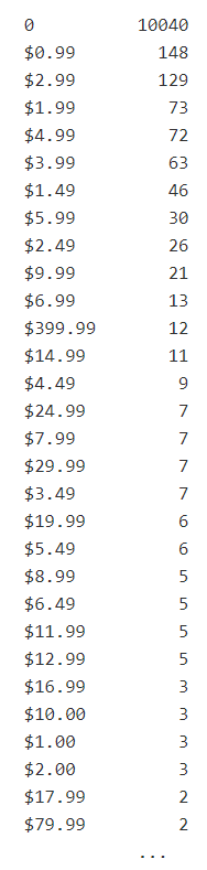
Retrieve number of instances of each unique price value:
df.Price.value_counts()
First let's remove the dollar signs and convert all values to floats (from strings)
def clean_usd(s):
	if isinstance(s, str):
    	s = s.replace('$', '')
	return float(s)

df['Price'] = df.Price.apply(lambda x: clean_usd(x))
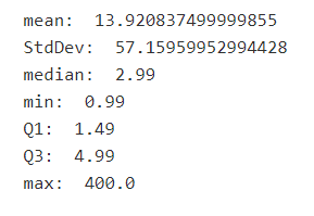
Inspect mean, standard deviation, IQR, find outlier candidates in Price variable (the numeric_summary function I use several times throughout the notebook).
def numeric_summary(series):
	print('mean: ', np.mean(series))
	print('StdDev: ', np.std(series))
	print('median: ', np.median(series))
	print('min: ', min(series))
	print('Q1: ', series.quantile(.25))
	print('Q3: ', series.quantile(.75))
	print('max: ', max(series))

numeric_summary(df.loc[df.Price != 0].Price)
df.loc[(df.Price > 12) & (df.Install_bins == 0)]
plt.hist(df.loc[(df.Price < 20) & (df.Price > 0)].Price, bins=80)
plt.xticks(np.arange(0, 20, step=.5))
plt.title('Histogram of 0 < Price < 20', size=20)
plt.show()
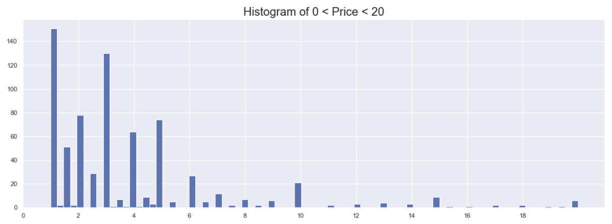
Note peaks at prices .99, 1.99, 2.99, 3.99, 4.99, etc. (Especially at .99, 2.99, 4.99, 9.99, 14.99, 19.99) and to a lesser extent the ~.49's as well. 0.49 itself is nonexistent.
plt.hist(df.loc[(df.Price < 50) & (df.Price > 0)].Price, bins=40)
plt.xticks(np.arange(0, 50, step=1))
plt.title('Histogram of 0 < Price < 50', size=20)
plt.show()
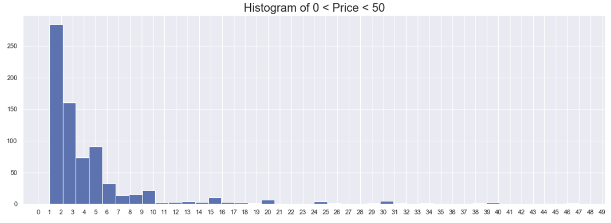
There are legit mini-clusters of apps at 19.99, 24.99 and 29.99, so we'll try putting them in the last bound group I think.
# Similar to what we did with Installs, except Price is actually continuous
df.loc[df['Price'] == 0, 'Price_Group'] = '0.00'
df.loc[(df['Price'] > 0) & (df['Price'] <= 0.99), 'Price_Group'] = '0.01-0.99'
df.loc[(df['Price'] > 0.99) & (df['Price'] <= 2.99), 'Price_Group']   = '1-2.99'
df.loc[(df['Price'] > 2.99) & (df['Price'] <= 4.99), 'Price_Group']   = '3-4.99'
df.loc[(df['Price'] > 4.99) & (df['Price'] <= 9.99), 'Price_Group']   = '5-9.99'
df.loc[(df['Price'] > 9.99) & (df['Price'] <= 14.99), 'Price_Group']   = '10-14.99'
df.loc[(df['Price'] > 14.99) & (df['Price'] <= 29.99), 'Price_Group']   = '15-29.99'
df.loc[(df['Price'] > 29.99), 'Price_Group']  = '30+'
So obviously we do the above and more for each of our variables where there is cleaning or feature engineering to be done. For 'Price' we've noted the significant peaks, the tendency toward prices ending in .99 and .49, the major right skew no matter how far you zoom out, and the few outliers that we have in the hundreds of dollars. We've also created a new categorical feature that classifies app price into bins, labeled 'Price_Group', that may serve as a helpful feature when we work on creating a model. We have the liberty to modify this feature later on of course, as modeling is an iterative process and we may, for instance, change the price group definitions during the modeling phase as we test different features and combinations. Basically, it's a process that we gradually build on as we learn more about our data and is always subject to change.
EDA Part 3 - Intervariate Relationships & Correlations
# Useful Python3:

DATAFRAME.corr()

seaborn.FacetGrid()
seaborn.heatmap(), .pairplot(), .catplot()
seaborn.regplot(), .jointplot(), .distplot()
This is the time where we finally get to do a lot of visualization back-to-back. We'll first get a glimpse of our correlation matrix, and then dive in further to scrutinize relationships between variables, and in particular the relationships between the target variable and others.
I will note that more of what I look at when investigating datasets is just statistical values; basically tables and numbers with adequate visualizations when I feel like zooming out and looking at something with a wider lense. But for the sake of visual appeal, I'll emphasize the visualizations a little more in these articles, where I can.
sns.set(style="white")
# numerics = ['Rating', 'Reviews', 'Price', 'Size_bytes', 'Install_bins', 'Major_Ver', 'Min_Android_Major_Ver', 'Days_Since_Update']
# Compute the correlation matrix
corr = df[numerics].corr()
# Generate a mask for the upper triangle
mask = np.triu(np.ones_like(corr, dtype=np.bool))
# Set up the matplotlib figure
f, ax = plt.subplots(figsize=(11, 9))
# Generate a custom diverging colormap
cmap = sns.diverging_palette(220, 10, as_cmap=True)
# Draw the heatmap with the mask and correct aspect ratio
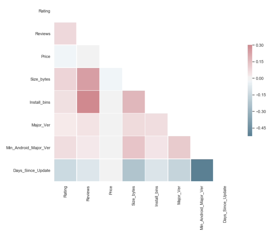
sns.heatmap(corr, mask=mask, cmap=cmap, vmax=.3, center=0,
square=True, linewidths=.5, cbar_kws={"shrink": .5})
corr
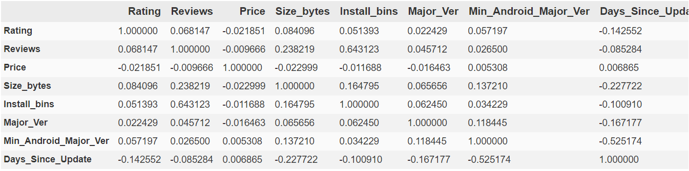
A few points to note:
- Notice Reviews and Install_bins are highly correlated. This makes sense as the more people installing and using the app the more reviews it'll naturally get, positive and negative.
- Reviews and Size also positively correlated. This makes sense since Size and Installs are positively correlated as well. This is not to say that larger apps are always better, but it stands to reason that popular apps used by a lot of people are popular because they can do more, and doing more I think we can agree would have a positive relationship with size (although I bet there's diminishing returns after a point).
- Keeping an eye on Major Version variable. It shows little correlation with anything, I think because we had almost everything with a Major_Ver of 1, and many of the higher values seemed arbitrary. I think we'll collapse some of the higher versions into one 9+ (or something) group after all.
- The Minimum Android Version has positive correlation with Size. So larger apps are more likely to have a higher minimun Android ver., i.e. they aren't supported by old versions, which makes sense. More recent, large and comp-heavy apps are more likely to only be compatible with recent Android software.
- Size & Reviews are positively correlated with Rating, Price and Days_Since_Update are negatively correlated (with Rating and everything). So in general price may in fact be a deterrent, and apps that aren't updated recently will probably also prove to be less popular
Variable Relationships with Target ('Rating')
Depending on just how many variables I have to work with, I may go ahead and look at distributions w.r.t. target (and other interesting variables) for every single one. That's not always practical or necessary, but it's simple to do with this skinny dataset.
An example of possible visualizations for one categorical and one numeric variable, with target..
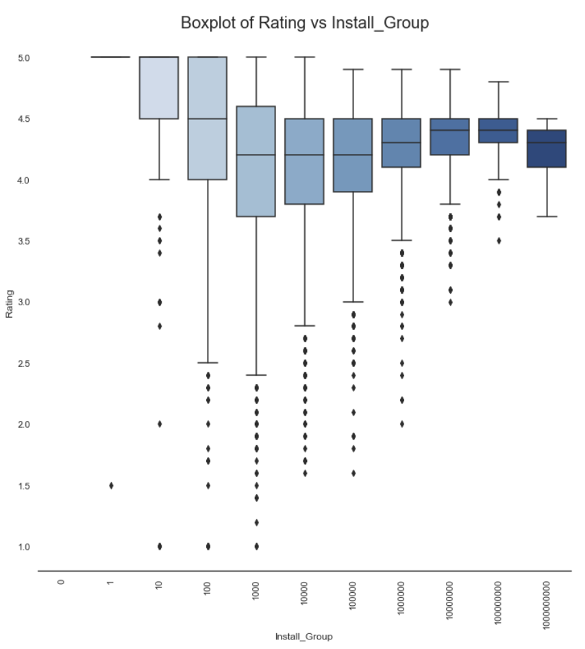
g = sns.catplot(x='Install_Group',y='Rating',data=df, kind="box", height=10, palette='Blues')
g.despine(left=True)
g.set_xticklabels(rotation=90)
g = g.set_ylabels('Rating')
plt.title('Boxplot of Rating vs Install_Group',size = 20)
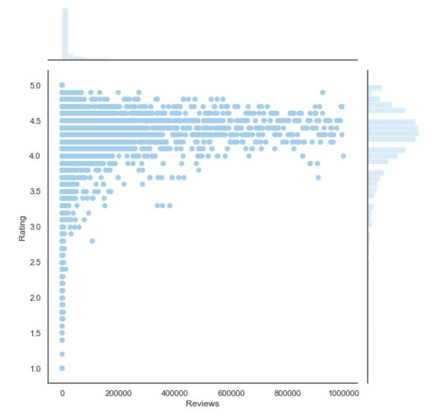
plt.figure(figsize = (10,10))
g = sns.jointplot(x='Reviews', y="Rating", color='skyblue', data=df[df.Reviews < 1000000], height=8)
Feature Preparation
I'll only go into this a little bit here, since the focus is supposed to be on the above EDA for this module, and I'll go into the modeling phase, etc. in its own article, but this is where we can do a few things, if we haven't already done them inadvertantly as part of the univariate inspections step:
- Add mean encodings
- Add advanced features (more feature engineering)
- Any remaining imputation (drop with nulls, values we can't handle with our model)
- One-hot and Label encodings
- Variable scaling and/or normalization
Below will be a few examples of preparation that could be used for a model predicting 'Rating' for Google Play apps based on this dataset. Again, this is just the start of a process to discover a good model. It's an iterative, trial-and-error process with no single "correct" solution. Often it's a balancing act between simplicity, adaptability, and accuracy.
In this case we start by reassessing the null values we have, and determine how to impute them (or whether to) remove some rows entirely.
Missing Values
For instance in preparing for the model to predict 'Rating', for this explicit purpose any rows with Rating missing won't be useful for us, so we can just remove them.
On the other hand we definitely do not want to remove all rows where app Size is missing (these were originally 'Varies with Device' instances in the raw data), as other information from these rows could be quite valuable in predicting Rating. So we'll come up with a strategy to impute by some other values, as exemplified below..
We'll need to decide how to deal with missing values and NaNs in each column.
To start, let's drop rows with the target var Rating missing
# df_trimmed.isnull().sum()
df_trimmed = df_trimmed[df_trimmed['Rating'].notna()]
The remaining missings come from where version and size were marked as 'Varies with Device'. We don't want to drop all these rows since other features could still be useful. Instead I think it makes sense to impute values and maybe add a boolean column indicating that this app has variable version/size.
We've seen that Major Ver was mostly 1 and Min Android ver was overwhelmingly 4, so I'm going to impute by the mode for each of these for now.
df_trimmed['Major_Ver'].fillna(value=1.0, inplace=True)
df_trimmed['Min_Android_Major_Ver'].fillna(value=4.0, inplace=True)
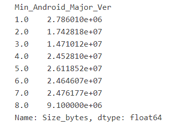
As for Size_bytes, I think we'll impute by a mean/median grouped by other variable(s) like Android version, just to be a little more precise than imputing by the overall mean, which might be excessively large for many apps.
df_trimmed.groupby('Min_Android_Major_Ver')['Size_bytes'].mean()
df_trimmed.groupby('Install_Group')['Size_bytes'].mean()
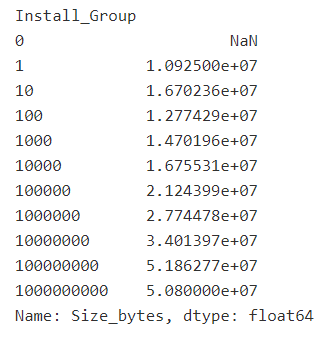
We see a bit more variation with Install_Group (apps with more installs tend to be on average larger than apps with fewer installs).
print('Difference: Overall InstallGroup proportions - NaN Size_bytes InstallGroup proportions:', \
	 df_trimmed['Install_Group'].value_counts() / len(df_trimmed) - \
	 df_trimmed[df_trimmed['Size_bytes'].isna()]['Install_Group'].value_counts() / len(df_trimmed[df_trimmed['Size_bytes'].isna()]))
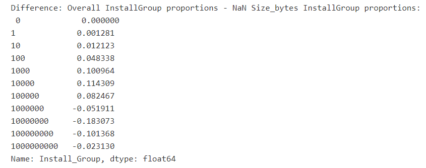
What we can see from the above is that larger install groups make up a larger proportion of all data when Size is missing than they do when Size exists. (negative differences as we go to larger groups, though actually the last group is not the most negative so it's not a perfect decline).
But anyway I think it's worth trying to impute Size with mean grouped by install group, seeing as there is a clear difference between means across groups and the variables are correlated.
df_trimmed['Size_bytes'] = df_trimmed.groupby('Install_Group')['Size_bytes'].transform(lambda x: x.fillna(x.mean())
df_trimmed.isnull().sum().sum()

Encodings
Now that we've dealt with missing values, etc., the next steps involve preprocessing our data so that it can actually be used in a model. For instance while tree-based algorithms may be able to handle categorical variables alright, for models from linear regression to neural nets we'll need to first encode the categoricals in some way, generally via one-hot or label encodings.
So for the last part of this module, we'll go ahead and look at performing basic categoricals encoding with sklearn.
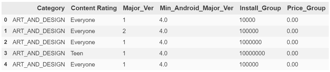
categoricals = df_trimmed.select_dtypes(include=['object', 'category'])
categoricals.head()
to_labels = df_trimmed[['Price_Group', 'Install_Group', 'Major_Ver', 'Min_Android_Major_Ver']]
to_onehot = df_trimmed[['Category', 'Content Rating']]
We have 2 kinds of categorical variables today:
- Ordered categoricals that we can label encode
- Price_Group
- Install_Group
- Major_Ver
- Min_Android_Major_Ver
- Categoricals with no meaningful order that we'd like to one-hot encode
- Category
- Content_Rating
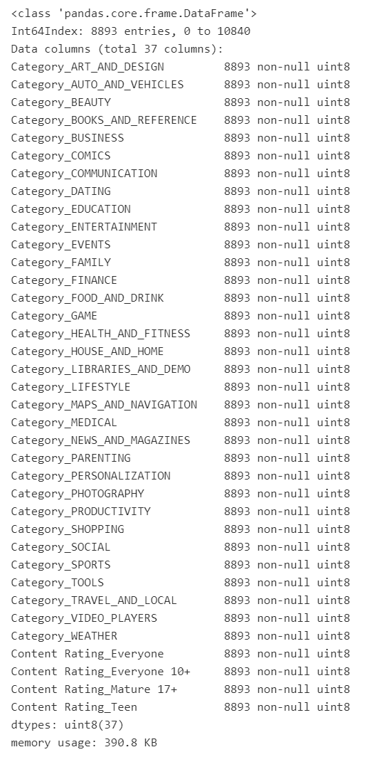
# One-hot Encodings
df_encoded = pd.get_dummies(to_onehot)
df_encoded.info()
# Label Encodings
from sklearn.preprocessing import LabelEncoder
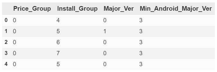
to_labels = to_labels.apply(LabelEncoder().fit_transform)
to_labels.head()
df_trimmed.drop(['Category', 'Content Rating', 'Price_Group',\
	'Install_Group', 'Major_Ver', 'Min_Android_Major_Ver'], axis=1, inplace=True)
df_encoded = pd.concat([df_trimmed, df_encoded, to_labels], axis=1, sort=False)
df_encoded.head()
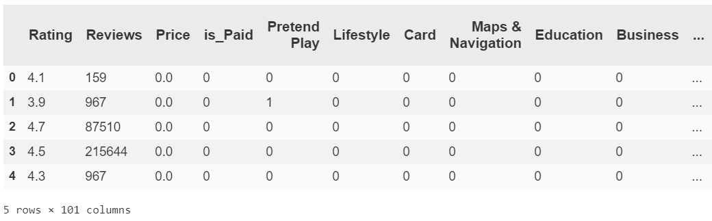
So you can see that all of our features now numeric. Either they were numeric to begin with or else we flattened categorical variables to a set of T/F features representable by 0 or 1.
The next steps, assuming we are happy with our features for now, are to scale numeric features and most likely normalize or standardize everything in order to start regression. However this post has gotten quite long, and also the approach to processes such as normalization are subject to change during the modeling phase (i.e. we may try out several strategies). I want to exemplify this iterative process of modeling, tweaking, rinse and repeat, so I'm going to give it its own article. It's not my top priority right now but hopefully I'll get it up soon.
This has been the EDA, feature engineering, and encodings portion of our GooglePlay data investigation. The whole runthrough with this dataset including encodings and soon modeling with sklearn can be found on my github, with annotations.