Datafluent

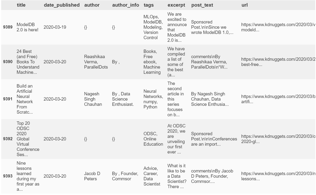
The Data

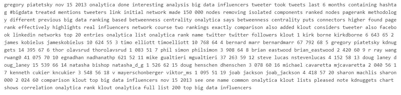
Again, this data comes from right where we left off in the web scraping module, KDNuggets Text Scraping. We have columns for article title, publish date, author and tags (when applicable), the excerpt or summary that comes at the beginning of most articles, url, and of course the body of the article, post_text.

While it's certainly interesting and maybe useful to look at title, author, etc., for this and the following module we won't care about any of that. We're going to be dealing with only the cleaning up of `post_text`, and some modifications to article `tags` today. This is in preparation for topic modeling based purely on post_text, and also maybe some supervised prediction of tags based on article text.

import numpy as np
import pandas as pd
from IPython.display import display, Math, Latex

articles.head()

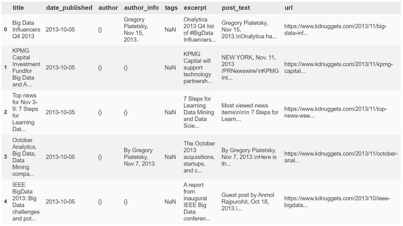
So we clearly have several interesting columns that we've collected, but today we're going to focus on the 'post_text' and 'tags' variables.

Ultimately we plan on doing some topic modeling and using this dataset to look at how an automated topic-tagging strategy might compare to tags actually used on articles. We know the results are not going to be similar; tags used on KDN articles are many and very specific to the content, and frankly tags and topics are not the same thing, nor should they be. However I'm curious to see what level of replicability we can reach by tweaking a topic model. E.g. if we increase the number of topics (with a relatively small dataset like this) can we get more specific topics or will we just start to see essentially repeated topics after a certain threshold.

My guess is the latter, but we'll see why and explain more in that module. This module today is a chance to look at the cleaning and a bit of preparing text for NLP that comes before feeding text data into a character or token-based model.

We also briefly prepare the 'tags' column since I want to try predicting tags with supervised learning as well. This part is somewhat unrelated to the main text cleaning so it'll be on github if it's not included below (for the sake of brevity).

articles.describe()

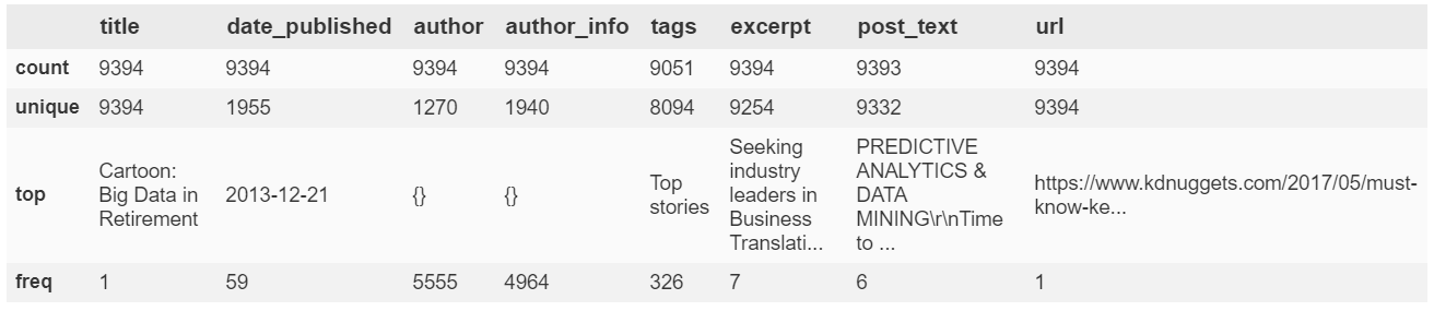
Note that there are duplicates of the excerpts and more significantly post_text. These are probably some regularly posted types like job openings. We did ensure not to include duplicates of title when we scraped the data.
There aren't so many unique authors but that's because over half of the articles didn't have a clear author or else it was not scraped correctly. Also a lot of the earlier articles were penned by the same person. It really doesn't matter seeing as I don't especially care about the author for this module.
urls are all unique, that's a good sanity check
Most of the tag combinations form a unique set, which means we'll probably be dropping and merging a great many tags (e.g. 'ML' and 'Machine Learning').

EDA Examples

Article Excerpt & Post Text

print('Mean length of excerpt:\n', int(np.round(articles['excerpt'].apply(lambda x: len(x)).mean())), 'characters.')

print('Mean length of post_text:\n', int(np.round(articles['post_text'].apply(lambda x: len(x)).mean())), 'characters.')

4883 actually already seems like a pretty reasonable length for an online article, but this value will decrease quite a bit after we remove js bits, newline characters, stopwords, etc. If you go look at a recent KDN article today I bet you're likely to find they're longer than the average we end up getting here. In addition to our removing of stopwords, etc., this is because recent articles are on average longer than past articles for KDNuggets (recently more contributors, more content, more to report on, larger user base, etc., I suppose).

text_series = articles['post_text']
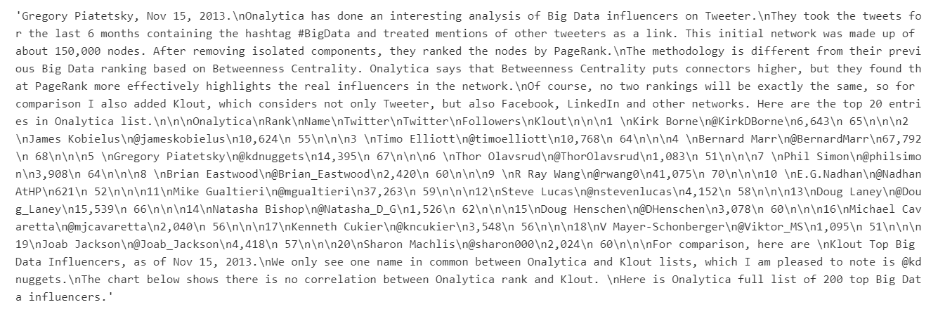
text_series[1]

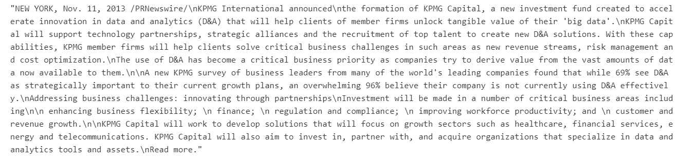
This is a relatively clean example it turns out, but you will notice we at least need to remove things like newline characters before using these post texts.

Most Common Tags

The following section is an example of some EDA we can do for article tags. We'll start by just getting an idea of what the tagging scheme is for this website. We want to know whether they use a few general tags that make post relationships clear and inter-article navigation easier, or whether tags are used in abundance and indicate very specifically what the post is about (or whether it's a mix of these).

When we ultimately build a model we want to limit the quantity of tags we consider if possible. Many many tags that just appear once or twice won't be helpful and will amount to noise in the end, so if there are tons of tags for every article we'll need to come up with our own strategy for condensing them.

# Let's explore the tags real quick
tags = articles['tags']
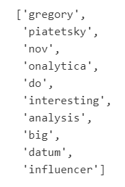
set(tags)

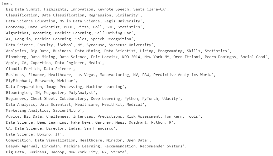
Just looking at the top of the tags, I'm gonna guess that we're dealing with a few categories of tags:

several very common tags like 'AI', 'Machine Learning', 'Data Science', 'Pandas', 'R', ...
some tags that come up less frequently but that may be common enough to be useful and indicate content such as 'Privacy', 'Self-Driving Car', 'LSTM', 'NIH'
a third group of tags that may helpful for content but occur infrequently in the scope of the whole dataset, like the names of startups and not-so-well-known technologies
tags that are not really of interest to us wrt what we want to train on, like the word 'Trends' or 'Faculty' or an author's name that occurs only once as a tag for some reason.

There are also lots of tags that are more or less duplicates of each other, like ML and 'Machine Learning', as noted above, that we'll end up combining as we ultimately try to decrease the number of unique tags we have to learn.

Keep in mind that that there are only tags starting in 2014.

Below, transforming our tags series into a list of lists of strings (one list for each article):

tags = [str(i) for i in tags]
print(tags[2000])
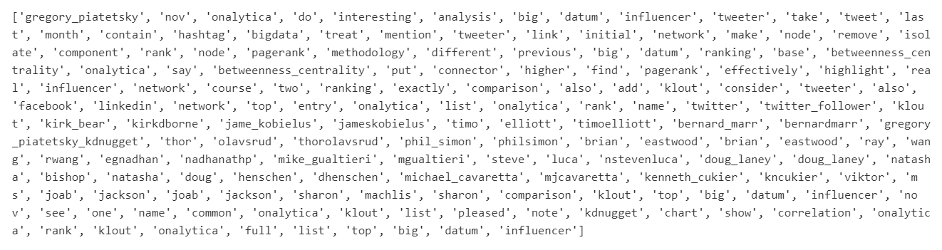
tags_split = [t.split(sep=', ') for t in tags]
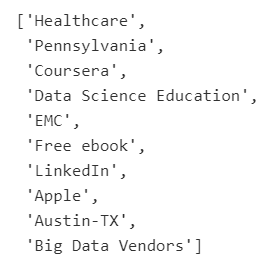
print(tags_split[2000])

Then we'll flatten into one list of tags so that we can build a quick frequency list (with Counter).

# Flatten tag lists into one long list of individual tags 
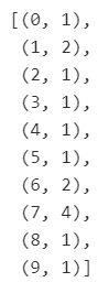
tags_flattened = [t for t_list in tags_split for t in t_list]
tags_flattened[2000:2010]

from collections import Counter

tags_counts = Counter(tags_flattened)
most_common_tags = sorted(tags_counts.items(), key=lambda x: x[1], reverse=True)[:10]

print(most_common_tags)

tag_counts = sorted(tags_counts.items(), key=lambda x: x[1], reverse=True)
common_tags_df = pd.DataFrame(tag_counts, columns=['Tag', 'Count'])
common_tags_df.head()

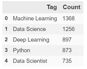
So we may have way too many tags in general, but it's reassuring to see that we do have several tags that could be used to determine overarching topics across many articles. I'm excited to compared these tags to parameters we get from our future topic models based on post_text.

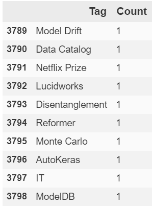
Below, a sample of the least common tags:

tags_df = pd.DataFrame(tag_counts, columns=['Tag', 'Count'])
tags_df.tail(10)

import matplotlib.pyplot as plt
import seaborn as sns
%matplotlib inline

fig = plt.figure()
fig.patch.set_facecolor('white')
n_top = 20

_ = sns.barplot('Tag', 'Count', data=tags_df[:n_top])
_ = plt.xlabel('Common Tags')
_ = plt.ylabel('Count')
_ = plt.xticks(rotation=45, ha='right', fontsize=11)
_ = plt.title('Top '+str(n_top)+' Most Common Tags')
plt.show()

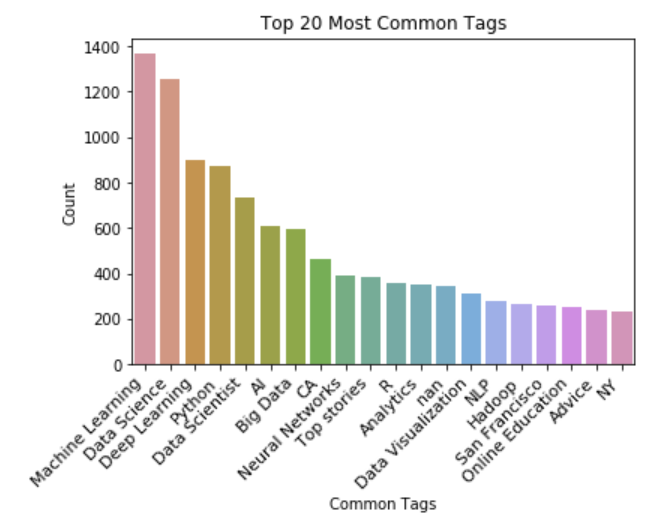
Most of these tags are exactly what you'd expect from a data science news source, right? Now the question for us is, when we create our topic model(s), will we see most if not all of the same words and phrases appear? Remember when we create our model it will be entirely based on 'post_text' alone, i.e. it will never see this 'tags' series.

Text Preparation for NLU

Text Cleaning

We'll now clean up our text. For these article bodies from raw html it involves a few important steps:

Removing the line breaks denoted by \r and \n
Removing symbols like brackets, commas, colons, '@', for instance we get a lot of twitter ids within this text.
Removing urls
Removing inline Javascript that occurs in some of the articles
Removing English stopwords
Setting all to lowercase*
Removing extra whitespace, whether originially in the text or introduced by our cleaning process

*May or may not modify this to retain uniqueness of certain named entities. e.g. the word 'data' vs. a company called 'Data, Inc.'. I think it's fine to lowercase everything because these sorts of named entities will mostly be picked up in our bi and trigrams if they really are common enough to matter.

import re
import nltk
nltk.download('stopwords')
from nltk.corpus import stopwords

LINEBREAKS_RE = re.compile('(\r\n|\r|\n)')
REPLACE_BY_SPACE_RE = re.compile('[/(){}\[\]\|@,;]')
BAD_SYMBOLS_RE = re.compile('([^0-9a-z #+_]|http\S+)')
STOPWORDS = set(stopwords.words('english'))

def text_prepare(text):
	"""
		text: a string
		
		return: modified initial string
	"""
	# remove javascript at the end of some articles:
	text = text.split("var disqus_shortname = 'kdnuggets'", 1)[0]
	# lowercase text
	text = text.lower() 
	# replace LINEBREAKS_RE by single spaces in text:
	text = re.sub(LINEBREAKS_RE, " ", text)  
	# replace REPLACE_BY_SPACE_RE symbols by space in text:
	text = re.sub(REPLACE_BY_SPACE_RE, " ", text) 
	# delete symbols which are in BAD_SYMBOLS_RE from text:
	text = re.sub(BAD_SYMBOLS_RE, "", text) 
	
	text = " " + text + " "
	# delete stopwords from text:
	for sw in STOPWORDS:
		text = text.replace(" "+sw+" ", " ") 
	
	text = re.sub('[ ][ ]+', " ", text)
	if text[0] == ' ':
		text = text[1:]
	if text[-1] == ' ':
		text = text[:-1]
		

	return text

Note - you'll find clean_text or whatever functions like this in pretty much any text cleaning tutorial you look at online. This is probably an amalgam of a few different approaches I've seen over the years, but just saying it's not original except for the part handling kdn's js.

# there was like one article that ended up not containing any text that would be semantically useful for us, so
articles = articles.loc[articles['post_text'] != '']

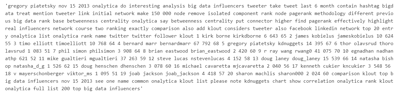
Before cleaning:

text_series[0]

After cleaning:

clean_text = [text_prepare(x) for x in text_series]
print(clean_text[0])

Another after example with fewer numbers:

print(clean_text[11])

I'd certainly consider whether to remove numbers, or at least numbers with more than 2 digits, like phone numbers and addresses, but keep in mind we're eventually going to be dropping certain unhelpful tokens anyway, most likely if they have a low tf-idf score or only occur like once in the dataset.

Lemmatization (with POS tagging)

Though I don't want this module to go too long, I did a comparison of a few methods of lemmatization with this text data, and we'll look at some results using just two packages below: TextBlob and Stanford CoreNLP.

# We'll do the final with Stanford CoreNLP if we notice improved quality, otherwise TextBlob is fine
from textblob import TextBlob, Word

# TextBlob implementation
def lemmatize_textblob(sentence):
	sent = TextBlob(sentence)
	tag_dict = {"J": 'a', 
				"N": 'n', 
				"V": 'v', 
				"R": 'r'}
	words_and_tags = [(w, tag_dict.get(pos[0], 'n')) for w, pos in sent.tags]
	lemmatized_list = [wd.lemmatize(tag) for wd, tag in words_and_tags]
	return " ".join(lemmatized_list)

sentence = "This is an excruciatingly confusing example sentence where the therapized coffee's mugs went to school"
lemmatize_textblob(sentence)

Notice simple lemmatizations are performed, but TextBlob ignores many complicated forms for English.

So we get "is" -> "be" , "coffee's" -> "coffee" + "'s", "mugs" -> "mug", "went" -> "go", but we miss the lemming of "an", "therapized" in this example.

# try with one post text example
lemmatize_textblob(clean_text[0])

# Stanford CoreNLP implementation
# Note: You'll need to start the server as well. See docs: https://stanfordnlp.github.io/CoreNLP/

from stanfordcorenlp import StanfordCoreNLP
import json, string

def lemmatize_corenlp(conn_nlp, sentence):
	properties = {
		'annotators': 'pos,lemma',
		'pipelineLanguage': 'en',
		'outputFormat': 'json'
	}

	# tokenize into words, rejoin
	tokens = conn_nlp.word_tokenize(sentence)
	tokens_joined = " ".join(tokens)

	# annotate to get lemma
	parsed_str = conn_nlp.annotate(tokens_joined, properties=properties)
	parsed_dict = json.loads(parsed_str)

	# extract lemma for each word
	lemma_list = [v for d in parsed_dict['sentences'][0]['tokens'] for k, v in d.items() if k == 'lemma']

	# rejoin and return lemmatized tokens
	return " ".join(lemma_list)


# make the connection and call lemmatize_corenlp
nlp = StanfordCoreNLP('http://localhost', port=9000, timeout=30000)
lemmatize_corenlp(conn_nlp=nlp, sentence=sentence)

We get a bit more out of CoreNLP for this sentence, although it won't always be so.

lemmatize_corenlp(nlp, clean_text[0])

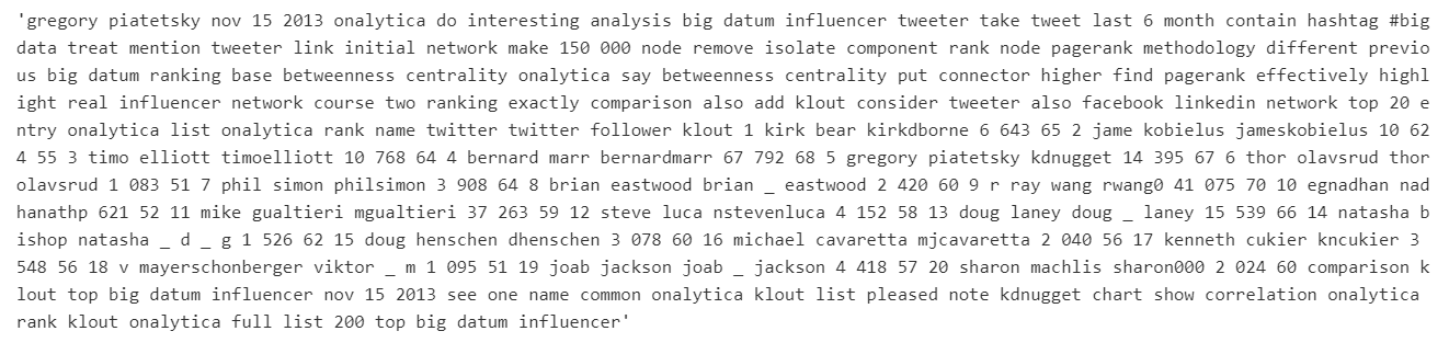
This is just showing one example from the dataset but generally I prefer CoreNLP to other packages for lemmatization and certain other techniques like NER. TextBlob is what I like to use when I am just testing something real quick or I'm lazy and don't feel like starting up the CoreNLP server, because textblob is also a good package.

The truth is you're never going to be perfect with stemming or lemmatization, because natural language is just so diverse and complex and there are so many exceptions to the rules. You can hardcode a certain number of common exceptions but it's not worth the trouble or bytes required. Plus even if you spend that much time on English, it's a similar investment to do the same for other languages if you need (although not all languages are as unneccessarily complex as English..).

Anyway the existing packages and methods are never perfect but work fairly well in practice, though each may have pros/cons depending on the situation.

lemmed_text = [lemmatize_corenlp(nlp, t) for t in clean_text]

# For quick access in the future
with open('kdn_lemmatized_text_corenlp.txt', 'w') as f:
    for t in lemmed_text:
        f.write("%s\n" % t)

Token Exploration

Once again I'm putting more on this webpage than I meant to, but I wanted to show a visualized "word count" for the most common tokens, similar to what we did with 'tags'.

# Count most common words in post texts
post_words = [word for text in clean_text for word in text.split()] 
words_counts = Counter(post_words)

word_counts = sorted(words_counts.items(), key=lambda x: x[1], reverse=True)
print(word_counts[:100])

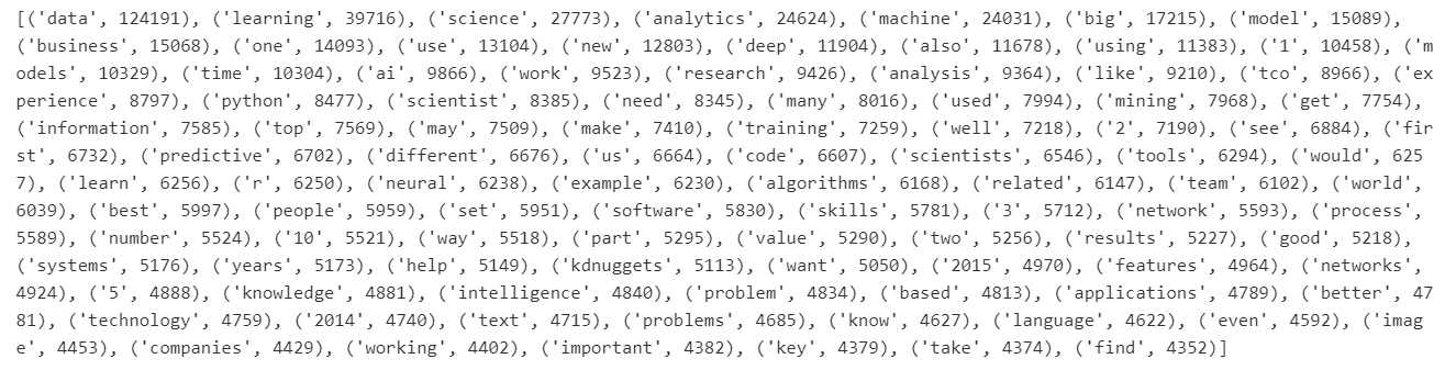
words_df = pd.DataFrame(word_counts, columns=['Word', 'Count'])
fig = plt.figure()
fig.patch.set_facecolor('white')
n_top = 20

_ = sns.barplot('Word', 'Count', data=words_df[:n_top])
_ = plt.xlabel('Common Words')
_ = plt.ylabel('Count')
_ = plt.xticks(rotation=45, fontsize=12)
_ = plt.title('Top '+str(n_top)+' Most Common Words')
plt.show()

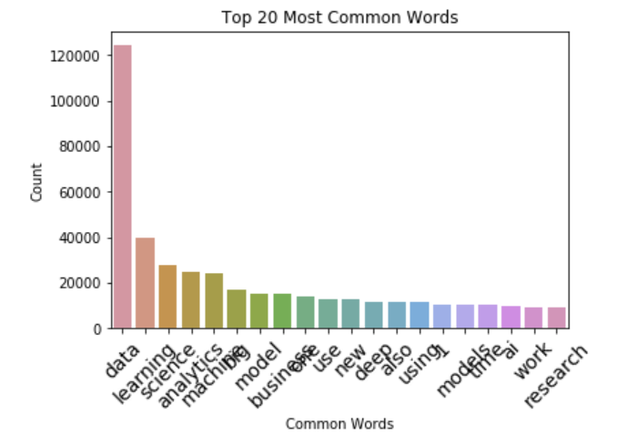
Ultimately we'll probably use something like BoW or ngrams-TFIDF for this dataset because those models are simpler and tend to work better when you have smaller datasets. For so few articles as this, a neural network like LSTM would probably be unnecessary. We'll save that tutorial for a tweets classification or something I might post later.

Gensim Doc & Token Prep

We'll finish this preparatory module with a first look at n-grams and Gensim's Phraser class. What comes below represents the lead-in to the next module where we'll actually employ n-grams in an LDA model, but the n-grams strategy we ultimately use for the model may be more fine-tuned than what we look at here today. In the next module we'll actually consider some extra dropout, etc.

But for now let's see how easy Gensim makes working with n-grams, the doc-term matrix, and corpora.

# Create token: id dictionary from text file (lemmatized docs)
import gensim
from gensim import corpora, models
from gensim.utils import simple_preprocess

f = 'kdn_lemmatized_text_corenlp.txt'
dtm = [simple_preprocess(line, deacc=False) for line in open(f, encoding='utf-8')]

# first 10 terms in 1st document (aka article) 
dtm[0][:10]

import warnings
warnings.filterwarnings('ignore')

# Build bigram and trigram models
bigram = gensim.models.Phrases(dtm, min_count=5, threshold=100)
trigram = gensim.models.Phrases(bigram[dtm], threshold=100)

# Faster to use Phraser class than raw Phrases()
bigram_mod = gensim.models.phrases.Phraser(bigram)
trigram_mod = gensim.models.phrases.Phraser(trigram)


# View 1,2,3-grams example
print(trigram_mod[bigram_mod[dtm[0]]])

Remember we're setting a min count and rather high threshold for the gensim Phrases, so not all possible instances will be merged into bi or trigrams. We don't want to use a much heavier model for the sake of terms that don't appear very often, particularly as this dataset will have a lot of infrequent names of people whom, to be blunt, we don't care about.

def make_bigrams(texts):
    return [bigram_mod[doc] for doc in texts]

def make_trigrams(texts):
	return [trigram_mod[bigram_mod[doc]] for doc in texts]

# Document-Term Matrix
dtm = make_trigrams(token_list)

# Token dictionary, {'token': tokenID} format
token_dict = corpora.Dictionary(dtm)

# Corpus, for each doc a list of tuples (bag of words) like (tokenID, frequency_in_doc)
corpus = [token_dict.doc2bow(d) for d in dtm]

# for instance:
corpus[0][:10]

So what we're calling 'corpus' here is just a bag of words for each doc (article text) we have. While I believe the preparation we finally do for our model will be slightly more involved than this, this is technically all we need in order to move on to the actual topic modeling stage of our project.

While I'll be throughly surprised if anyone somehow finds and reads this within a few days of my launching this website, if you're reading this I haven't yet posted the next module with topic modeling, but I'll link to it here and of course on the NLP page as soon as I finish annotating that notebook. Cheers.

Text Cleaning - KDNuggets Articles